Co-Analysis of AMP PDRD, GP2, & CRN Cloud Data

Summary/Overview

To support your explorations, each program offers “Getting Started” workspaces within Workbench, providing sample notebooks and guidance tailored to their respective datasets. This companion document outlines the specific steps and resources necessary to use the AMP PDRD, GP2, and CRN Cloud datasets together.

Workspaces and Data Resources
The following workspaces and data catalogs are available to support your explorations. These resources provide program-specific examples, documentation, and data references. The next sections, Using AMP PDRD and CRN Cloud Data Together and Using GP2 and CRN Cloud Data Together, provide step-by-step guidance for setting up your own workspace, incorporating data from these programs, and running analyses across your selected datasets.

AMP PDRD Resources 
Getting Started Workspaces

• Tier 1 – Clinical Access
• Tier 2 – Clinical and Omics Access
• Tier 2 – Autoantibodies
• Tier 2 – Proteomics

Data Catalogs

• Tier 1
  • Summary Data
  • Clinical Assessment Data
• Tier 2
  • Whole Genome Data
  • Transcriptomics Data
  • Targeted Proteomics Data
  • Untargeted Proteomics Data
  • Postmortem Sequencing Data

ASAP CRN Cloud Resources 
The ASAP CRN Cloud is a centralized platform designed for storing, analyzing, and sharing CRN 'omics data with the global research community. Its primary goals are to create an ecosystem for the curation and distribution of these datasets, promote reproducible science, and enable researchers to access and perform meta-analyses on harmonized data in one place. At the time of this pilot launch, the platform hosts a substantial collection of data derived from postmortem brain tissue, which can be explored through the data catalog linked below.

Getting Started Workspace

• ASAP CRN Reference Workspace

Data Catalogs

• ASAP CRN Cloud Data Catalog

Additional Resources

• ASAP CRN Cloud User Manual 

Before You Begin

In order to run the following example of AMP PDRD and ASAP CRN Cloud co-analysis, you will need to have access to both repositories, with a signed Data Use Agreement.  Registration for both programs must be done with the same Google account you are using to log into Verily Workbench. If you do not have access to both repositories, the following links provide instructions for registration:

• AMP PDRD Registration
• ASAP CRN User Manual

In addition to having access to both repositories, users must have access to billing configured in Verily workbench.  In Verily Workbench, Pods are created that are associated with cloud billing accounts, and when Workspaces and Data Collections are created, they are associated with Pods.  This allows any cloud service costs generated during the use of Verily Workbench to be charged to the correct billing account.

ASAP CRN Cloud and AMP PDRD have both made Pods available to users, and many organizations that use Verily Workbench will have billing accounts and Pods set up.  If you do not see any Pods available to use in Verily Workbench, contact your administration to determine how to request access. Please note that with the ASAP CRN Cloud and AMP PDRD programs providing pilot users access to the billing pods, we request that each pilot user is careful and cognizant of their intended cloud billing charges.  

For more information about how to set up billing with pods in verily workbench, please see the following link:

• Setting up billing with pods in Verily Workbench

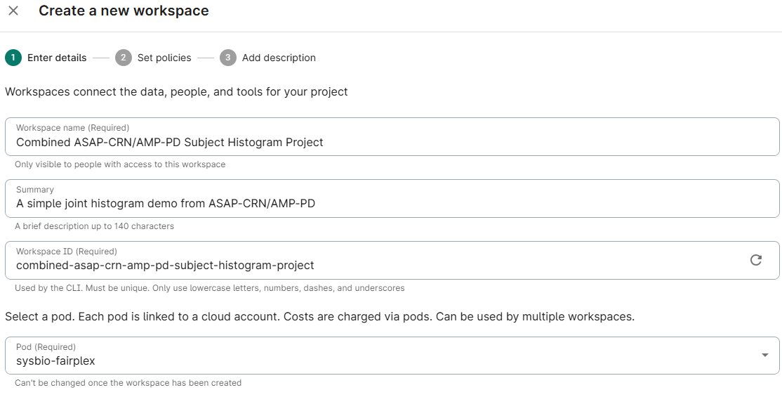
Create a New Workspace in Verily Workbench

Create your own new blank workspace and title it:

1. Assign a title and description, and select the pod you wish to associate this workspace with; click Next

   

2. Choose whether to limit access to groups
3. Select the bucket region for your workspace; click Next
4. Optionally add a description; click Create Workspace

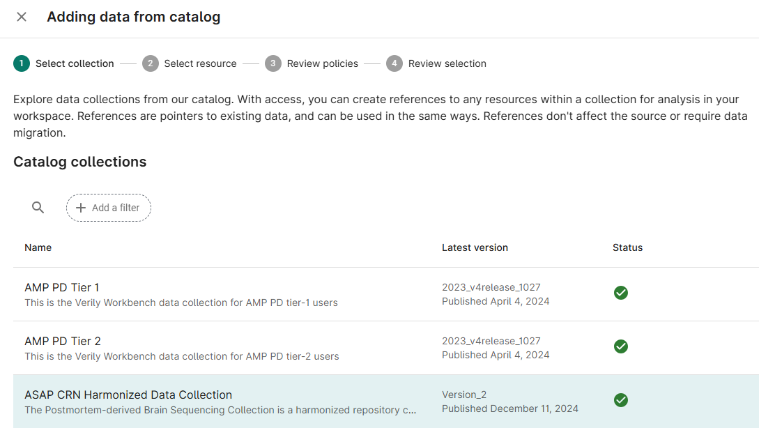
Add ASAP-CRN Resources to Workspace

Click the + Data from Catalog button

1. Select ASAP CRN Harmonized Data Collection from the list of available Collections; click Next

   

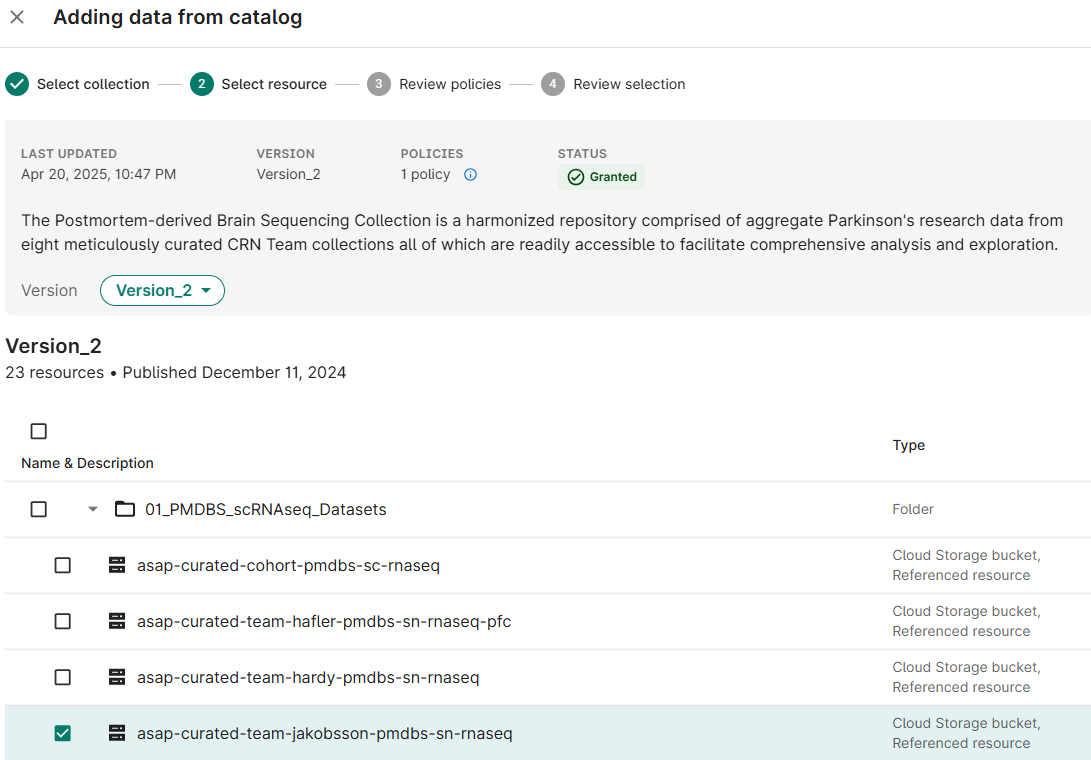
2. Select checkboxes for the Resource(s) needed for your analysis; click Next

   

3. Accept the policy acknowledgement statement; click Next
4. Choose Add to an existing Folder; click Add to your workspace

Add AMP-PD Resources to Workspace

Click the + Data from Catalog button

1. Select Pilot - AMP PD Tier 1 from the list of available Collections; click Next

2. Select checkboxes for the Resource(s) needed for your analysis (gs_path_amp_pd_tier1_release); click Next

   

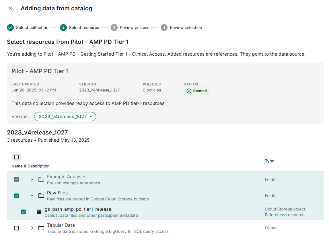
3. (If prompted) Accept the policy acknowledgement statement; click Next
4. Choose Add to an existing Folder; click Add to your workspace

Select Files for Analysis

From AMP-PD Resource

Select the AMP-PD resource and choose Browse from the info panel

1. Navigate to the clinical folder; click Demographics
2. Click Add as reference from the info panel
3. Accept defaults; click Add to resources
4. (Optionally) Choose additional resources
5. Click Close to return to the Resources page

From ASAP-CRN Resource

Select the ASAP-CRN resource and choose Browse from the info panel

1. Navigate to the metadata → release folder of any dataset; click SUBJECT
2. Click Add as reference from the info panel
3. Accept defaults; click Add to resources
4. (Optionally) Choose additional resources
5. Click Close to return to the Resources page

Create an Output Bucket

From the Resources tab, click + New Resource

1. Select New Cloud Storage Bucket

   

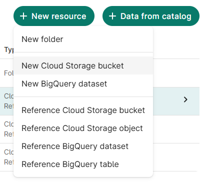
2. Assign resource ID; click Create bucket

Create a Virtual Machine to Run Analysis

From the Apps tab, click New app instance, select JupyterLab; click Next

1. Choose Default configuration; click Next
2. (Optionally) Reduce Machine Type to n1-standard-1

3. (Optionally) Reduce Data disk size to 100 GB

   

4. Accept defaults; click Next
5. Review and confirm the app summary; click Create App
6. (Note) This step may take several minutes

Create a Notebook for Combined Analysis

From the Apps tab, Launch the newly created virtual machine

1. In the JupyterLab Interface that opens, click the Folder Icon in the left menu bar
2. In the file browser panel, select the Output Bucket you created earlier.
3. In the bucket contents section, right click and select New Notebook
4. Select Python 3 (local) kernel type; click Next

Configure Notebook to Analyse Selected Resources

Import Required Libraries

    # Use the os package to interact with the environment

    import os


    # Bring in Pandas for Dataframe functionality

    import pandas as pd


    # Use StringIO for working with file contents

    from io import StringIO


    # Enable IPython to display matplotlib graphs.

    import matplotlib.pyplot as plt

    %matplotlib inline

Create Utility Routines

    # Utility routines for reading files from Google Cloud Storage

    def gcs_read_file(path):

       """Return the contents of a file in GCS"""

       contents = !gsutil -u {BILLING_PROJECT_ID} cat {path}

       return '\n'.join(contents)

Read GCS Locations from Workspace Resources

    # Get the GCP billing project ID from workbench environment variables

    OUTPUT = !wb utility execute env | grep "GOOGLE_CLOUD_PROJECT" | cut -d"=" -f2

    BILLING_PROJECT_ID = OUTPUT[0]


    # Get the AMP PD Demographics file location from workbench environment variables

    OUTPUT = !wb resource resolve --name=Demographics-csv

    GS_AMP_PD_DATA_PATH = OUTPUT[0]


    # Get the ASAP CRN Subject file location from workbench environment variables

    OUTPUT = !wb resource resolve --name=SUBJECT-csv

    GS_ASAP_CRN_DATA_PATH = OUTPUT[0]


    print(f'BILLING_PROJECT_ID = {BILLING_PROJECT_ID}')

    print(f'GS_AMP_PD_DATA_PATH = {GS_AMP_PD_DATA_PATH}')

    print(f'GS_ASAP_CRN_DATA_PATH = {GS_ASAP_CRN_DATA_PATH}')

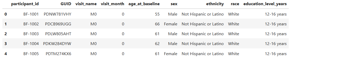
Read AMP PD Demographics Data

    # Read CSV file from GCS into dataframe

    amp_pd_demographics_df = pd.read_csv(StringIO(gcs_read_file(GS_AMP_PD_DATA_PATH)), engine='python', index_col=False)


    amp_pd_demographics_df.head()

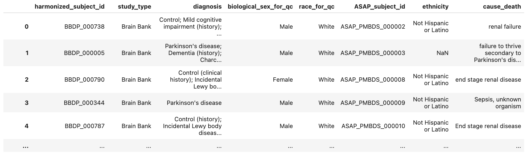
Read ASAP CRN Subject Data

    # Read CSV file from GCS into dataframe

    asap_crn_subjects_df = pd.read_csv(StringIO(gcs_read_file(GS_ASAP_CRN_DATA_PATH)), engine='python', index_col=[0])


    asap_crn_subjects_df.head()

Harmonize and Merge AMP PD and ASAP CRN Data

    # rename columns to harmonize data

    amp_pd_demographics_df.rename(columns={'participant_id': 'harmonized_subject_id', 'age_at_baseline': 'harmonized_age'}, inplace=True)


    asap_crn_subjects_df.rename(columns={'subject_id': 'harmonized_subject_id', 'age_at_collection': 'harmonized_age'}, inplace=True)


    # Concatenate dataframes to create new harmonized dataframe

    harmonized_df = pd.concat([amp_pd_demographics_df, asap_crn_subjects_df])


    harmonized_df

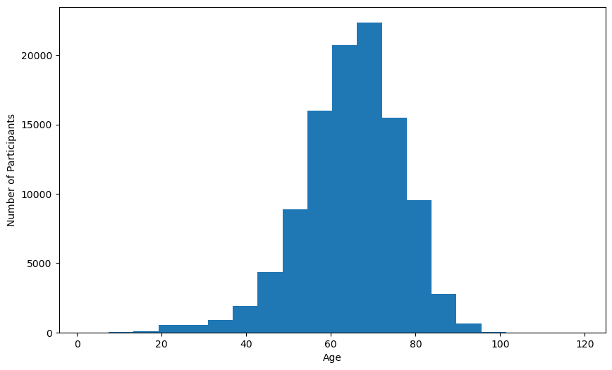
Create Age Distribution Bar Chart

    # Configure plot

    fig = plt.figure()

    fig.set_figheight(6)

    fig.set_figwidth(10)


    # Create plot

    plt.hist(harmonized_df['harmonized_age'].dropna(), bins=20)

    plt.xlabel('Age')

    plt.ylabel('Number of Participants')

    plt.show()

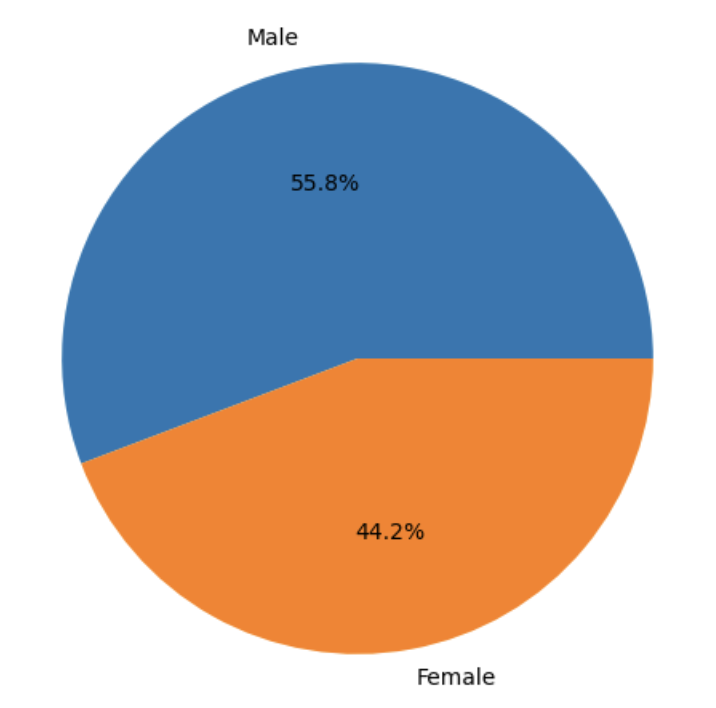
Create Sex Distribution Pie Chart

    # Configure plot

    counts_by_sex = harmonized_df['sex'].value_counts()


    fig = plt.figure()

    fig.set_figheight(6)

    fig.set_figwidth(10)


    # Create plot

    plt.pie(counts_by_sex.values, labels=counts_by_sex.index, autopct="%1.1f%%")

    plt.figure(figsize=(10, 6))

    plt.show()

     

Before You Begin

In order to run the following example of GP2 and ASAP CRN Cloud co-analysis, you will need to have access to both repositories, with a signed Data Use Agreement. Registration for both programs must be done with the same Google account you are using to log into Verily Workbench. Access to GP2 data is granted through AMP PDRD Registration. If you do not have access to both repositories, the following links provide instructions for registration:

• AMP PDRD Registration
• ASAP CRN User Manual

In addition to having access to both repositories, users must have access to billing configured in Verily workbench. In Verily Workbench, Pods are created that are associated with cloud billing accounts, and when Workspaces and Data Collections are created, they are associated with Pods. This allows any cloud service costs generated during the use of Verily Workbench to be charged to the correct billing account.

GP2 has a billing Pod available for users who are part of an approved GP2 project. If you do not see any Pods available to use in Verily Workbench, contact your administration to determine how to request access.

For more information about how to set up billing with pods in verily workbench, please see the following link:

• Setting up billing with pods in Verily Workbench

To browse projects currently approved by GP2 and to apply for an approved GP2 project please see the following links:

• GP2 Hub: Projects
• GP2 Project Proposal Form

Create a New Workspace in Verily Workbench

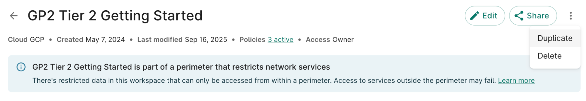
Per GDPR compliance requirements, GP2 data can only be accessed within a perimeter. In order to use GP2 data, your workspace must be created in or added to the perimeter. This can be done by creating a workspace by duplicating the available GP2 Tier 1 or Tier 2 official Getting Started workspaces or by creating a new workspace configured with the required regional and access controls.

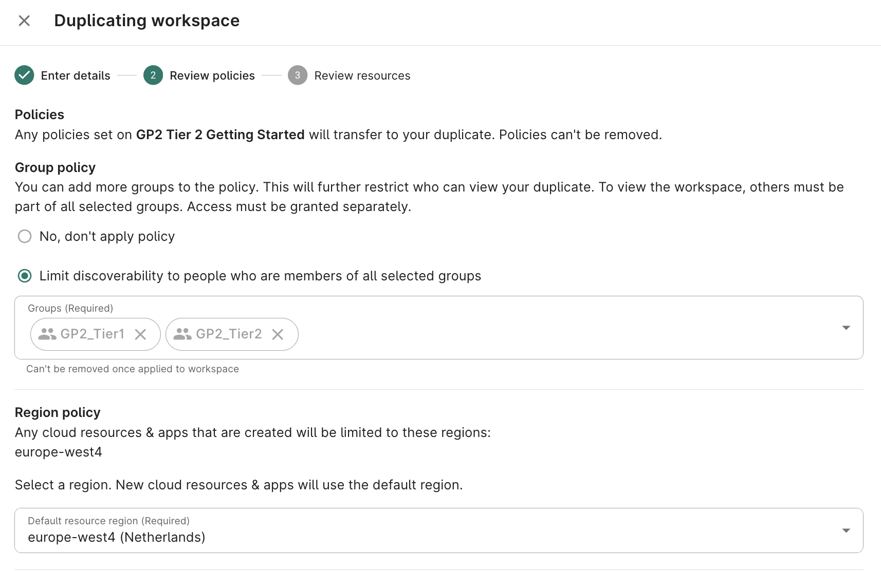
To populate GP2 data in a new workspace, the workspace must be created in the europe-west4 (Netherlands) region, and a permission policy must be applied that restricts visibility and access to members of the appropriate GP2 access group (GP2_tier1 or GP2_tier2). Workspaces created outside the europe-west4 region or without the required permission policy will not be eligible to host GP2 data. 

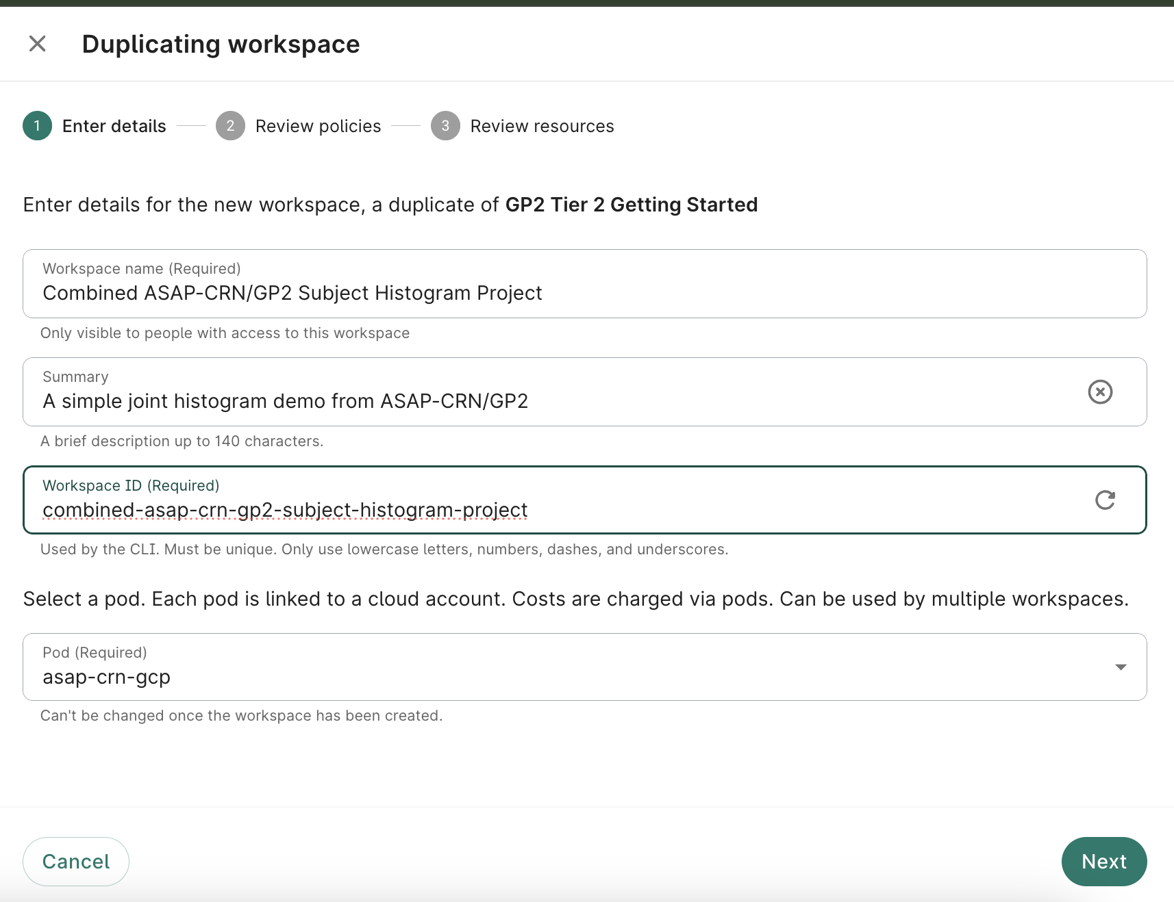
From the Getting Started workspaces, select the Duplicate option

Duplicate the workspace and title it:

1. Assign a title and description, and select the pod you wish to associate this workspace with; click Next

   

2. Ensure access is limited to GP2_Tier1 and GP2_Tier2 groups

3. Select europe-west4 (Netherlands) as the bucket region; click Next

   

4. Optionally add a description; click Create Workspace

Add ASAP-CRN Resources to Workspace

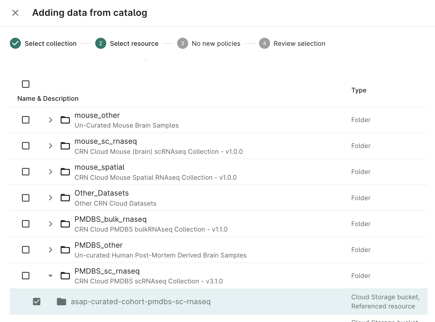
Click the + Data from Catalog button

1. Select ASAP CRN Harmonized Data Collection from the list of available Collections; click Next

2. Select checkboxes for the Resource(s) needed for your analysis; click Next

   

3. Accept the policy acknowledgement statement; click Next
4. Choose Add to an existing Folder; click Add to your workspace
    

Select Files for Analysis

From ASAP-CRN Resource

Select the ASAP-CRN resource and choose Browse from the info panel

1. Navigate to the metadata → release folder of any dataset; click CLINPATH
2. Click Add as reference from the info panel
3. Accept defaults; click Add to resources
4. (Optionally) Choose additional resources
5. Click Close to return to the Resources page
    

Create an Output Bucket

From the Resources tab, click + New Resource

1. Select New Cloud Storage Bucket

   

2. Assign resource ID; click Create bucket

Create a Virtual Machine to Run Analysis

From the Apps tab, click New app instance, select JupyterLab; click Next

1. Choose Default configuration; click Next
2. (Optionally) Reduce Machine Type to n1-standard-1

3. (Optionally) Reduce Data disk size to 100 GB

   

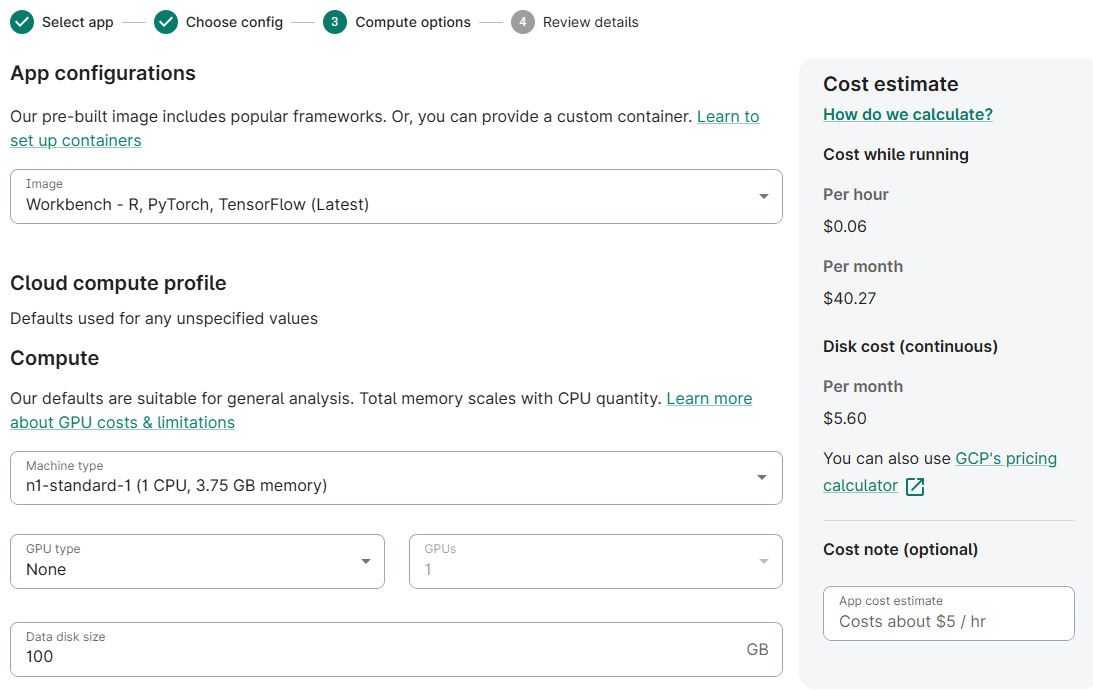
4. Accept defaults; click Next
5. Review and confirm the app summary; click Create App
6. (Note) This step may take several minutes

Create a Notebook for Combined Analysis

From the Apps tab, Launch the newly created virtual machine

1. In the JupyterLab Interface that opens, click the Folder Icon in the left menu bar
2. In the file browser panel, select the Output Bucket you created earlier.
3. In the bucket contents section, right click and select New Notebook
4. Select Python 3 (local) kernel type; click Next
    

Configure Notebook to Analyse Selected Resources

Import Required Libraries

    # Use the os package to interact with the environment

    import os


    # Bring in Pandas for Dataframe functionality

    import pandas as pd


    # Use StringIO for working with file contents

    from io import StringIO


    # Enable IPython to display matplotlib graphs.

    import matplotlib.pyplot as plt

    %matplotlib inline

Create Utility Routines

    # Utility routines for reading files from Google Cloud Storage

    def gcs_read_file(path):

       """Return the contents of a file in GCS"""

       contents = !gsutil -u {BILLING_PROJECT_ID} cat {path}

       return '\n'.join(contents)

Read GCS Locations from Workspace Resources

    # Get the GCP billing project ID from workbench environment variables

    OUTPUT = !wb utility execute env | grep "GOOGLE_CLOUD_PROJECT" | cut -d"=" -f2

    BILLING_PROJECT_ID = OUTPUT[0]


    # Get the ASAP CRN Subject file location from workbench environment variables

    OUTPUT = !wb resource resolve --name=CLINPATH-csv

    GS_ASAP_CRN_DATA_PATH = OUTPUT[0]


    print(f'BILLING_PROJECT_ID = {BILLING_PROJECT_ID}')

    print(f'GS_ASAP_CRN_DATA_PATH = {GS_ASAP_CRN_DATA_PATH}')

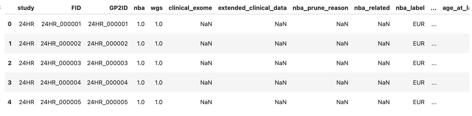
Read GP2 Data

    # Read CSV file from GCS into dataframe

    gp2_data_df = pd.read_csv("workspace/gp2_tier2_eu_release11/clinical_data/master_key_release11_final_vwb.csv", low_memory=False)

    gp2_data_df.head()

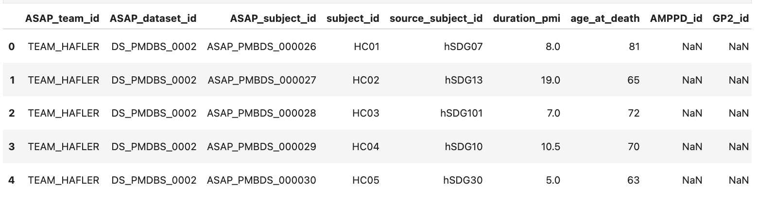
Read ASAP CRN Subject Data

    # Read CSV file from GCS into dataframe

    asap_crn_subjects_df = pd.read_csv(StringIO(gcs_read_file(GS_ASAP_CRN_DATA_PATH)), engine='python', index_col=[0])


    asap_crn_subjects_df.head()

Harmonize and Merge AMP PD and ASAP CRN Data

    # rename columns to harmonize data

    gp2_data_df.rename(columns={'GP2ID': 'harmonized_subject_id', 'age_at_sample_collection': 'harmonized_age'}, inplace=True)


    #removing trailing S1 in GP2 ID for asap cn metadata

    asap_crn_clinpath_df['harmonized_subject_id'] = (

       asap_crn_clinpath_df['harmonized_subject_id']

           .str.replace(r'^(MDGAP.*)_s1$', r'\1', regex=True)

    )


    asap_crn_clinpath_df.rename(columns={'GP2_id': 'harmonized_subject_id', 'age_at_collection': 'harmonized_age'}, inplace=True)


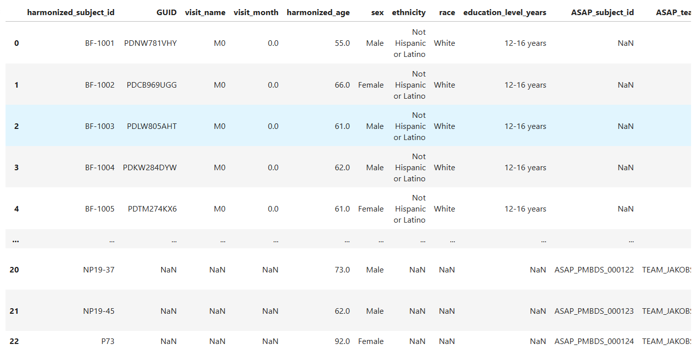
    # Concatenate dataframes to create new harmonized dataframe

    harmonized_df = pd.concat([gp2_data_df, asap_crn_clinpath_df])


    harmonized_df.head()

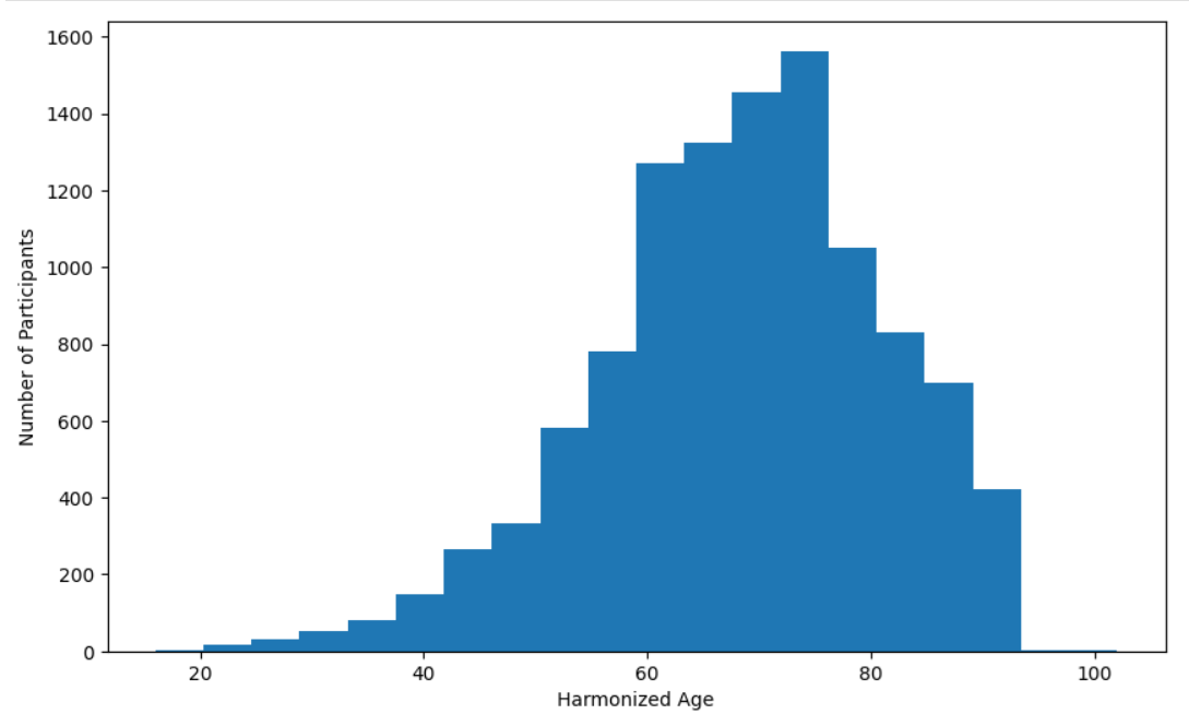
Create Age Distribution Bar Chart

    # Configure plot

    fig = plt.figure()

    fig.set_figheight(6)

    fig.set_figwidth(10)


    # Create plot

    plt.hist(harmonized_df['harmonized_age'].dropna(), bins=20)

    plt.xlabel('Age')

    plt.ylabel('Number of Participants')

    plt.show()

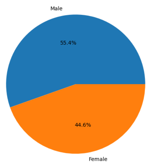
Create Sex Distribution Pie Chart

    # Configure plot

    counts_by_sex = harmonized_df['biological_sex_for_qc'].value_counts()


    fig = plt.figure()

    fig.set_figheight(6)

    fig.set_figwidth(10)


    # Create plot

    plt.pie(counts_by_sex.values, labels=counts_by_sex.index, autopct="%1.1f%%")

    plt.figure(figsize=(10, 6))

    plt.show()